
Métricas
Una métrica es una función que define una distancia entre cada par de elementos de un conjunto. Para nuetro caso, se define una función de distancia entre los valores reales (\(y\)) y los valores predichos (\(\hat{y}\)).
Defeniremos algunas métricas bajo dos tipos de contexto: modelos de regresión y modelos de clasificación.
Métricas para Regresión
Sabemos que los modelos de regresión buscan ajustar un modelo a valores numéricos que no reprensentan etiquetas. La idea es cuantificar el error y seleccionar el mejor modelo. El error corresponde a la diferencia entre el valor original y el valor predicho, es decir:
Lo que se busca es medir el error bajo cierta funciones de distancias o métricas. Dentro de las métricas más populares se encuentran:
Métricas absolutas: Las métricas absolutas o no escalada miden el error sin escalar los valores. Las métrica absolutas más ocupadas son:
Mean Absolute Error (MAE)
\[\textrm{MAE}(y,\hat{y}) = \dfrac{1}{n}\sum_{t=1}^{n}\left | y_{t}-\hat{y}_{t}\right |\]Mean squared error (MSE):
\[\textrm{MSE}(y,\hat{y}) =\dfrac{1}{n}\sum_{t=1}^{n}\left | y_{t}-\hat{y}_{t}\right |^2\]Métricas Porcentuales: Las métricas porcentuales o escaladas miden el error de manera escalada, es decir, se busca acotar el error entre valores de 0 a 1, donde 0 significa que el ajuste es perfecto, mientras que 1 sería un mal ajuste. Cabe destacar que muchas veces las métricas porcentuales puden tener valores mayores a 1.
Mean absolute percentage error (MAPE):
\[\textrm{MAPE}(y,\hat{y}) = \dfrac{1}{n}\sum_{t=1}^{n}\left | \frac{y_{t}-\hat{y}_{t}}{y_{t}} \right |\]Symmetric mean absolute percentage error (sMAPE):
\[\textrm{sMAPE}(y,\hat{y}) = \dfrac{1}{n}\sum_{t=1}^{n} \frac{\left |y_{t}-\hat{y}_{t}\right |}{(\left | y_{t} \right |^2+\left | \hat{y}_{t} \right |^2)/2}\]
Métricas para Clasificación
Sabemos que los modelos de clasificación etiquetan a los datos a partir del entrenamiento. Por lo tanto es necesario introducir nuevos conceptos.
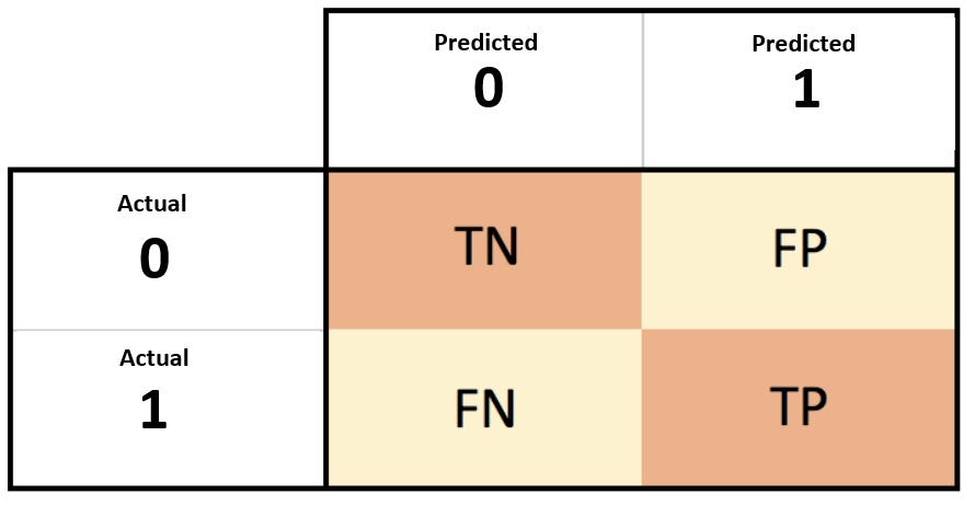
Uno de ellos es la matriz de confusión. Típicamente para un clasificador binario se tiene:
TP: Verdadero PositivoFN: Falso NegativoFP: Falso positivoTN: Verdadero Negativo
En este contexto, los valores TP y TN muestran los valores correctos que tuve al momento de realizar la predicción, mientras que los valores de de FN y FP denotan los valores en que la clasificación fue errónea.
Una manera eficaz de visualizar estos resultados es con la matriz de confusión
El siguiente ejemplo resolverá todas tus dudas

En un princpio se busca maximizar la suma de los elementos bien clasificados, sin embargo eso depende mucho del problema a resolver. Para esto se definen las siguientes métricas:
Accuracy:
\[\textrm{accuracy}= \frac{TP+TN}{TP+TN+FP+FN}\]Recall:
\[\textrm{recall} = \frac{TP}{TP+FN}\]Precision:
\[\textrm{precision} = \frac{TP}{TP+FP} \]F-score:
\[\textrm{F_score} = 2\times \frac{ \textrm{precision} \times \textrm{recall} }{ \textrm{precision} + \textrm{recall} } \]
Estas son las más comunes, y como te imaginarás, scikit-learn tiene toda una artillería de selección de modelos en este link.
Ejemplo
import matplotlib.pyplot as plt
import numpy as np
import pandas as pd
from sklearn.datasets import load_breast_cancer
from sklearn.model_selection import train_test_split
from sklearn.linear_model import LogisticRegression

%matplotlib inline
breast_cancer = load_breast_cancer()
print(breast_cancer.DESCR)
.. _breast_cancer_dataset:

Breast cancer wisconsin (diagnostic) dataset
--------------------------------------------

**Data Set Characteristics:**

    :Number of Instances: 569

    :Number of Attributes: 30 numeric, predictive attributes and the class

    :Attribute Information:
        - radius (mean of distances from center to points on the perimeter)
        - texture (standard deviation of gray-scale values)
        - perimeter
        - area
        - smoothness (local variation in radius lengths)
        - compactness (perimeter^2 / area - 1.0)
        - concavity (severity of concave portions of the contour)
        - concave points (number of concave portions of the contour)
        - symmetry
        - fractal dimension ("coastline approximation" - 1)

        The mean, standard error, and "worst" or largest (mean of the three
        worst/largest values) of these features were computed for each image,
        resulting in 30 features.  For instance, field 0 is Mean Radius, field
        10 is Radius SE, field 20 is Worst Radius.

        - class:
                - WDBC-Malignant
                - WDBC-Benign

    :Summary Statistics:

    ===================================== ====== ======
                                           Min    Max
    ===================================== ====== ======
    radius (mean):                        6.981  28.11
    texture (mean):                       9.71   39.28
    perimeter (mean):                     43.79  188.5
    area (mean):                          143.5  2501.0
    smoothness (mean):                    0.053  0.163
    compactness (mean):                   0.019  0.345
    concavity (mean):                     0.0    0.427
    concave points (mean):                0.0    0.201
    symmetry (mean):                      0.106  0.304
    fractal dimension (mean):             0.05   0.097
    radius (standard error):              0.112  2.873
    texture (standard error):             0.36   4.885
    perimeter (standard error):           0.757  21.98
    area (standard error):                6.802  542.2
    smoothness (standard error):          0.002  0.031
    compactness (standard error):         0.002  0.135
    concavity (standard error):           0.0    0.396
    concave points (standard error):      0.0    0.053
    symmetry (standard error):            0.008  0.079
    fractal dimension (standard error):   0.001  0.03
    radius (worst):                       7.93   36.04
    texture (worst):                      12.02  49.54
    perimeter (worst):                    50.41  251.2
    area (worst):                         185.2  4254.0
    smoothness (worst):                   0.071  0.223
    compactness (worst):                  0.027  1.058
    concavity (worst):                    0.0    1.252
    concave points (worst):               0.0    0.291
    symmetry (worst):                     0.156  0.664
    fractal dimension (worst):            0.055  0.208
    ===================================== ====== ======

    :Missing Attribute Values: None

    :Class Distribution: 212 - Malignant, 357 - Benign

    :Creator:  Dr. William H. Wolberg, W. Nick Street, Olvi L. Mangasarian

    :Donor: Nick Street

    :Date: November, 1995

This is a copy of UCI ML Breast Cancer Wisconsin (Diagnostic) datasets.
https://goo.gl/U2Uwz2

Features are computed from a digitized image of a fine needle
aspirate (FNA) of a breast mass.  They describe
characteristics of the cell nuclei present in the image.

Separating plane described above was obtained using
Multisurface Method-Tree (MSM-T) [K. P. Bennett, "Decision Tree
Construction Via Linear Programming." Proceedings of the 4th
Midwest Artificial Intelligence and Cognitive Science Society,
pp. 97-101, 1992], a classification method which uses linear
programming to construct a decision tree.  Relevant features
were selected using an exhaustive search in the space of 1-4
features and 1-3 separating planes.

The actual linear program used to obtain the separating plane
in the 3-dimensional space is that described in:
[K. P. Bennett and O. L. Mangasarian: "Robust Linear
Programming Discrimination of Two Linearly Inseparable Sets",
Optimization Methods and Software 1, 1992, 23-34].

This database is also available through the UW CS ftp server:

ftp ftp.cs.wisc.edu
cd math-prog/cpo-dataset/machine-learn/WDBC/

.. topic:: References

   - W.N. Street, W.H. Wolberg and O.L. Mangasarian. Nuclear feature extraction
     for breast tumor diagnosis. IS&T/SPIE 1993 International Symposium on
     Electronic Imaging: Science and Technology, volume 1905, pages 861-870,
     San Jose, CA, 1993.
   - O.L. Mangasarian, W.N. Street and W.H. Wolberg. Breast cancer diagnosis and
     prognosis via linear programming. Operations Research, 43(4), pages 570-577,
     July-August 1995.
   - W.H. Wolberg, W.N. Street, and O.L. Mangasarian. Machine learning techniques
     to diagnose breast cancer from fine-needle aspirates. Cancer Letters 77 (1994)
     163-171.
Como siempre, obtengamos nuestra matriz de diseño y vector de respuesta
X, y = breast_cancer.data, breast_cancer.target
X_train, X_test, y_train, y_test = train_test_split(X, y, test_size=.3, random_state=42)
np.unique(y)
array([0, 1])
target_names = breast_cancer.target_names
target_names
array(['malignant', 'benign'], dtype='<U9')
Ajustemos un modelo de regresión logística a los datos
clf = LogisticRegression(max_iter=1000, n_jobs=-1)
clf.fit(X_train, y_train)
y_pred = clf.predict(X_test)
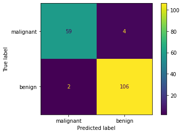
Rápidamente podemos visualizar la matriz de confusión
from sklearn.metrics import plot_confusion_matrix
plot_confusion_matrix(clf, X_test, y_test, display_labels=target_names)
plt.show()
Como también calcular algunas métricas
from sklearn.metrics import accuracy_score, recall_score, f1_score

print(f"Accuracy score: {accuracy_score(y_test, y_pred):0.2f}")
print(f"Recall score: {recall_score(y_test, y_pred):0.2f}")
print(f"F1 score: {f1_score(y_test, y_pred):0.2f}")
Accuracy score: 0.96
Recall score: 0.98
F1 score: 0.97
Incluso tener un reporte mucho más rápido
from sklearn.metrics import classification_report
print(classification_report(y_test, y_pred, target_names=breast_cancer.target_names))
              precision    recall  f1-score   support

   malignant       0.97      0.94      0.95        63
      benign       0.96      0.98      0.97       108

    accuracy                           0.96       171
   macro avg       0.97      0.96      0.96       171
weighted avg       0.96      0.96      0.96       171
Otra métrica interesante es Average Precision (AP), la cual no es más que un promedio ponderado de la precisión alcanzada en cada umbral (threshold)
donde \(P_n\) y \(R_n\) son precision y recall correspondientes al \(n\)-ésimo umbral.
from sklearn.metrics import average_precision_score

print(f'Average precision-recall score: {average_precision_score(y_test, y_pred):0.2f}')
Average precision-recall score: 0.96
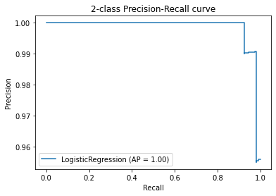
Pero donde uno puede sacar mucho provecho es con un gráfico que nos muestre la relación entre precision y recall a medida que varía el umbral
from sklearn.metrics import plot_precision_recall_curve, precision_recall_curve

disp = plot_precision_recall_curve(clf, X_test, y_test)
disp.ax_.set_title(f'2-class Precision-Recall curve');
Internamente, los umbrales del estimador varían y utiliza la predicción en probabilidad del estimador.
clf.predict_proba(X_test)
array([[1.69988501e-01, 8.30011499e-01],
       [9.99999996e-01, 3.62463514e-09],
       [9.98802281e-01, 1.19771939e-03],
       [2.51913453e-03, 9.97480865e-01],
       [6.68242794e-04, 9.99331757e-01],
       [1.00000000e+00, 1.53880282e-10],
       [1.00000000e+00, 1.18163585e-12],
       [9.84182268e-01, 1.58177321e-02],
       [3.89809208e-03, 9.96101908e-01],
       [7.30615615e-03, 9.92693844e-01],
       [8.06603018e-02, 9.19339698e-01],
       [9.99592400e-01, 4.07599984e-04],
       [9.48166745e-03, 9.90518333e-01],
       [9.24157467e-01, 7.58425332e-02],
       [1.69750105e-03, 9.98302499e-01],
       [9.99108347e-01, 8.91653103e-04],
       [1.71640557e-03, 9.98283594e-01],
       [1.75266610e-04, 9.99824733e-01],
       [1.88183508e-04, 9.99811816e-01],
       [9.99999962e-01, 3.83669412e-08],
       [1.35478925e-01, 8.64521075e-01],
       [1.49268921e-02, 9.85073108e-01],
       [1.00000000e+00, 2.28684440e-10],
       [3.01170002e-03, 9.96988300e-01],
       [1.04666310e-02, 9.89533369e-01],
       [4.81350812e-04, 9.99518649e-01],
       [1.75535594e-03, 9.98244644e-01],
       [9.80365116e-03, 9.90196349e-01],
       [7.10892433e-03, 9.92891076e-01],
       [9.99999998e-01, 2.24323390e-09],
       [5.79216191e-03, 9.94207838e-01],
       [6.91006835e-04, 9.99308993e-01],
       [7.72703088e-03, 9.92272969e-01],
       [1.57004345e-02, 9.84299565e-01],
       [1.04286702e-03, 9.98957133e-01],
       [3.45676977e-03, 9.96543230e-01],
       [9.97505085e-01, 2.49491491e-03],
       [2.39590406e-03, 9.97604096e-01],
       [9.99996612e-01, 3.38798074e-06],
       [2.97051581e-01, 7.02948419e-01],
       [1.63318538e-03, 9.98366815e-01],
       [9.99450806e-01, 5.49194220e-04],
       [1.48799776e-03, 9.98512002e-01],
       [1.00632925e-02, 9.89936708e-01],
       [1.24314426e-03, 9.98756856e-01],
       [4.84093323e-02, 9.51590668e-01],
       [5.39863117e-04, 9.99460137e-01],
       [5.16920274e-03, 9.94830797e-01],
       [8.70537341e-02, 9.12946266e-01],
       [3.06487411e-03, 9.96935126e-01],
       [9.99948251e-01, 5.17492792e-05],
       [1.00000000e+00, 3.26061185e-10],
       [1.65952892e-01, 8.34047108e-01],
       [5.72722969e-04, 9.99427277e-01],
       [1.13774359e-03, 9.98862256e-01],
       [2.14055860e-02, 9.78594414e-01],
       [2.03859991e-03, 9.97961400e-01],
       [1.00000000e+00, 1.47018811e-14],
       [3.41971739e-01, 6.58028261e-01],
       [2.88482212e-04, 9.99711518e-01],
       [1.98383970e-02, 9.80161603e-01],
       [9.99999946e-01, 5.35703710e-08],
       [1.00000000e+00, 4.76878707e-12],
       [8.48850877e-02, 9.15114912e-01],
       [4.42166385e-03, 9.95578336e-01],
       [1.79290853e-01, 8.20709147e-01],
       [9.99994811e-01, 5.18902967e-06],
       [1.00000000e+00, 2.46087735e-10],
       [2.24566908e-03, 9.97754331e-01],
       [1.89176289e-02, 9.81082371e-01],
       [9.78154355e-01, 2.18456454e-02],
       [9.99966505e-01, 3.34946010e-05],
       [2.35079620e-03, 9.97649204e-01],
       [9.28103603e-01, 7.18963973e-02],
       [7.10560133e-03, 9.92894399e-01],
       [2.44445031e-03, 9.97555550e-01],
       [5.39880590e-02, 9.46011941e-01],
       [4.91683482e-01, 5.08316518e-01],
       [9.00573317e-04, 9.99099427e-01],
       [3.14988477e-03, 9.96850115e-01],
       [9.99342206e-01, 6.57793846e-04],
       [1.57009495e-03, 9.98429905e-01],
       [4.36201981e-01, 5.63798019e-01],
       [1.00000000e+00, 4.17173127e-12],
       [9.99010946e-01, 9.89053993e-04],
       [9.83691033e-01, 1.63089674e-02],
       [9.99481902e-01, 5.18098177e-04],
       [9.99999937e-01, 6.27644758e-08],
       [6.27569387e-03, 9.93724306e-01],
       [3.99923941e-03, 9.96000761e-01],
       [1.41308223e-02, 9.85869178e-01],
       [9.68693147e-02, 9.03130685e-01],
       [1.46287044e-01, 8.53712956e-01],
       [4.06825786e-03, 9.95931742e-01],
       [1.19798496e-03, 9.98802015e-01],
       [1.21600903e-03, 9.98783991e-01],
       [9.99999985e-01, 1.45974419e-08],
       [9.99999457e-01, 5.43359806e-07],
       [1.87004476e-04, 9.99812996e-01],
       [9.99951638e-01, 4.83623213e-05],
       [9.99908034e-01, 9.19655636e-05],
       [5.90506585e-05, 9.99940949e-01],
       [9.99999999e-01, 1.13158236e-09],
       [9.98726805e-01, 1.27319476e-03],
       [6.10000466e-02, 9.38999953e-01],
       [6.08555033e-02, 9.39144497e-01],
       [1.56446921e-02, 9.84355308e-01],
       [1.00000000e+00, 4.94743699e-18],
       [2.08411396e-02, 9.79158860e-01],
       [1.05207936e-01, 8.94792064e-01],
       [9.99811117e-01, 1.88882517e-04],
       [2.74067442e-03, 9.97259326e-01],
       [8.86429618e-01, 1.13570382e-01],
       [1.00000000e+00, 1.48029680e-29],
       [4.62139296e-02, 9.53786070e-01],
       [1.00000000e+00, 1.03308444e-11],
       [3.96990518e-04, 9.99603009e-01],
       [9.66301668e-02, 9.03369833e-01],
       [5.70467310e-04, 9.99429533e-01],
       [9.99302009e-01, 6.97991400e-04],
       [8.41930812e-01, 1.58069188e-01],
       [1.32861023e-03, 9.98671390e-01],
       [1.03353461e-02, 9.89664654e-01],
       [9.99970590e-01, 2.94102270e-05],
       [6.38275717e-02, 9.36172428e-01],
       [9.99999999e-01, 1.06638024e-09],
       [9.99317682e-01, 6.82317905e-04],
       [8.80822814e-03, 9.91191772e-01],
       [3.28488431e-03, 9.96715116e-01],
       [9.99999993e-01, 6.97304401e-09],
       [1.00000000e+00, 1.59563281e-14],
       [9.99805111e-01, 1.94888759e-04],
       [1.18699116e-01, 8.81300884e-01],
       [1.92688122e-03, 9.98073119e-01],
       [2.29309498e-02, 9.77069050e-01],
       [9.62491235e-01, 3.75087652e-02],
       [8.21057258e-02, 9.17894274e-01],
       [4.85385248e-03, 9.95146148e-01],
       [1.18793691e-01, 8.81206309e-01],
       [9.93801907e-01, 6.19809291e-03],
       [7.90524312e-03, 9.92094757e-01],
       [1.00000000e+00, 3.66063244e-15],
       [2.38990535e-04, 9.99761009e-01],
       [1.86757573e-04, 9.99813242e-01],
       [9.83924924e-01, 1.60750760e-02],
       [1.27600691e-02, 9.87239931e-01],
       [9.99998199e-01, 1.80105122e-06],
       [9.99999833e-01, 1.66965340e-07],
       [7.40450103e-01, 2.59549897e-01],
       [3.66769320e-03, 9.96332307e-01],
       [9.82851053e-01, 1.71489475e-02],
       [5.69281777e-04, 9.99430718e-01],
       [5.07418097e-04, 9.99492582e-01],
       [4.65490405e-02, 9.53450959e-01],
       [1.69483229e-02, 9.83051677e-01],
       [1.00000000e+00, 7.03536320e-17],
       [9.99791394e-01, 2.08605865e-04],
       [6.45600989e-03, 9.93543990e-01],
       [4.99167548e-03, 9.95008325e-01],
       [1.71036077e-04, 9.99828964e-01],
       [1.86843791e-06, 9.99998132e-01],
       [4.76243427e-03, 9.95237566e-01],
       [2.87859314e-03, 9.97121407e-01],
       [3.97720449e-03, 9.96022796e-01],
       [9.64388985e-01, 3.56110154e-02],
       [5.61796005e-03, 9.94382040e-01],
       [6.08543920e-04, 9.99391456e-01],
       [3.32291827e-01, 6.67708173e-01],
       [7.30668962e-03, 9.92693310e-01],
       [9.62876021e-01, 3.71239787e-02],
       [2.60064876e-02, 9.73993512e-01]])