Clasificación
Los modelos de regresión asumen que la variable de respuesta es cuantitativa, sin embargo, en muchas situaciones esta variable es cualitativa/categórica, por ejemplo el color de ojos. La idea de predecir variables categóricas es usualmente nombrada como Clasificación. Muchos de los problemas en los que se enfoca el Machine Learning están dentro de esta categoría, por lo mismo existen una serie de algoritmos y modelos con tal de obtener los mejores resultados. En esta clase introduciremos el algoritmo de clasificación más sencillo: Regresión Logística.
Motivación
Para comprender mejor los algoritmos de clasificación se comenzará con un ejemplo.
Space Shuttle Challege
28 Junio 1986. A pesar de existir evidencia de funcionamiento defectuoso, se da luz verde al lanzamiento.

A los 73 segundos de vuelo, el transbordador espacial explota, matando a los 7 pasajeros.

Como parte del debriefing del accidente, se obtuvieron los siguientes datos
%cat ../data/Challenger.txt
"Temp"	"BadRings"
53	3
56	1
57	1
63	0
66	0
67	0
67	0
67	0
68	0
69	0
70	0
70	1
70	1
70	1
72	0
73	0
75	0
75	2
76	0
76	0
78	0
79	0
80	0
81	0
Es posible graficarlos para tener una idea general de estos.
import numpy as np
import pandas as pd
import altair as alt
import matplotlib.pyplot as plt

from pathlib import Path

alt.themes.enable('opaque')  # Para quienes utilizan temas oscuros en Jupyter Lab/Notebook

%matplotlib inline
filepath = Path().resolve().parent / "data" / "Challenger.txt"
challenger = pd.DataFrame(
    np.loadtxt(filepath, skiprows=1).astype(np.int),
    columns=["temp_f", "nm_bad_rings"]
)
challenger.head()
| temp_f | nm_bad_rings | |
|---|---|---|
| 0 | 53 | 3 |
| 1 | 56 | 1 |
| 2 | 57 | 1 |
| 3 | 63 | 0 |
| 4 | 66 | 0 |
alt.Chart(challenger).mark_circle(size=100).encode(
    x=alt.X("temp_f", scale=alt.Scale(zero=False), title="Temperature [F]"),
    y=alt.Y("nm_bad_rings", title="# Bad Rings")
).properties(
    title="Cantidad de fallas vs temperatura en lanzamiento de Challenger",
    width=600,
    height=400
)
Nos gustaría saber en qué condiciones se produce accidente. No nos importa el número de fallas, sólo si existe falla o no.
# Un poco de procesamiento de datos
challenger = challenger.assign(
    temp_c=lambda x: ((x["temp_f"] - 32.) / 1.8).round(2),
    is_failure=lambda x: x["nm_bad_rings"].ne(0).astype(np.int),
    ds_failure=lambda x: x["is_failure"].map({1: "Falla", 0:"Éxito"})
)
challenger.head()
| temp_f | nm_bad_rings | temp_c | is_failure | ds_failure | |
|---|---|---|---|---|---|
| 0 | 53 | 3 | 11.67 | 1 | Falla |
| 1 | 56 | 1 | 13.33 | 1 | Falla |
| 2 | 57 | 1 | 13.89 | 1 | Falla |
| 3 | 63 | 0 | 17.22 | 0 | Éxito |
| 4 | 66 | 0 | 18.89 | 0 | Éxito |
failure_chart = alt.Chart(challenger).mark_circle(size=100).encode(
    x=alt.X("temp_c:Q", scale=alt.Scale(zero=False), title="Temperature [C]"),
    y=alt.Y("is_failure:Q", scale=alt.Scale(padding=0.5), title="Success/Failure"),
    color="ds_failure:N"
).properties(
    title="Exito o Falla en lanzamiento de Challenger",
    width=600,
    height=400
)

failure_chart
Regresión Logística
Recordemos que la Regresión Lineal considera un modelo de la siguiente forma:
donde $\( Y = \begin{bmatrix}y^{(1)} \\ y^{(2)} \\ \vdots \\ y^{(m)}\end{bmatrix} \qquad , \qquad X = \begin{bmatrix} 1 & x^{(1)}_1 & \dots & x^{(1)}_n \\ 1 & x^{(2)}_1 & \dots & x^{(2)}_n \\ \vdots & \vdots & & \vdots \\ 1 & x^{(m)}_1 & \dots & x^{(m)}_n \end{bmatrix} \qquad y \qquad \theta = \begin{bmatrix}\theta_1 \\ \theta_2 \\ \vdots \\ \theta_m\end{bmatrix} \)$
y que se entrenar una función lineal
deforma que se minimice
La Regresión Logística busca entrenar la función
de forma que se minimice
Es decir, el objetivo es encontrar un “buen” vector \(\theta\) de modo que
en donde \(g(z)\) es la función sigmoide (sigmoid function),
Función Sigmoide
def sigmoid(z):
    return 1 / (1 + np.exp(-z))
z = np.linspace(-5,5,100)
sigmoid_df_tmp = pd.DataFrame(
    {
        "z": z,
        "sigmoid(z)": sigmoid(z),
        "sigmoid(z*2)": sigmoid(z * 2),
        "sigmoid(z-2)": sigmoid(z - 2),
    }
)
sigmoid_df = pd.melt(
    sigmoid_df_tmp,
    id_vars="z",
    value_vars=["sigmoid(z)", "sigmoid(z*2)", "sigmoid(z-2)"],
    var_name="sigmoid_function",
    value_name="value"
)
sigmoid_df.head()
| z | sigmoid_function | value | |
|---|---|---|---|
| 0 | -5.00000 | sigmoid(z) | 0.006693 |
| 1 | -4.89899 | sigmoid(z) | 0.007399 |
| 2 | -4.79798 | sigmoid(z) | 0.008179 |
| 3 | -4.69697 | sigmoid(z) | 0.009040 |
| 4 | -4.59596 | sigmoid(z) | 0.009992 |
alt.Chart(sigmoid_df).mark_line().encode(
    x="z:Q",
    y="value:Q",
    color="sigmoid_function:N"
).properties(
    title="Sigmoid functions",
    width=600,
    height=400
)
La función sigmoide \(g(z) = (1+e^{-z})^{-1}\) tiene la siguiente propiedad:
“Demostración”:
def d_sigmoid(z):
    return sigmoid(z) * (1 - sigmoid(z))

sigmoid_dz_df = (
    pd.DataFrame(
        {
            "z": z,
            "sigmoid(z)": sigmoid(z),
            "d_sigmoid(z)/dz": d_sigmoid(z)
        }
    )
    .melt(
        id_vars="z",
        value_vars=["sigmoid(z)", "d_sigmoid(z)/dz"],
        var_name="function"
    )
)


sigmoid_dz_df.head()
| z | function | value | |
|---|---|---|---|
| 0 | -5.00000 | sigmoid(z) | 0.006693 |
| 1 | -4.89899 | sigmoid(z) | 0.007399 |
| 2 | -4.79798 | sigmoid(z) | 0.008179 |
| 3 | -4.69697 | sigmoid(z) | 0.009040 |
| 4 | -4.59596 | sigmoid(z) | 0.009992 |
alt.Chart(sigmoid_dz_df).mark_line().encode(
    x="z:Q",
    y="value:Q",
    color="function:N"
).properties(
    title="Sigmoid and her derivate function",
    width=600,
    height=400
)
¡Es perfecta para encontrar un punto de corte y clasificar de manera binaria!
Implementación
Aproximación Ingenieril
¿Cómo podemos reutilizar lo que conocemos de regresión lineal?
Si buscamos minimizar $\(J(\theta) = \frac{1}{2} \sum_{i=1}^{m} \left( h_{\theta}(x^{(i)}) - y^{(i)}\right)^2\)\( Podemos calcular el gradiente y luego utilizar el método del máximo descenso para obtener \)\theta$.
El cálculo del gradiente es directo:
¿Hay alguna forma de escribir todo esto de manera matricial? Recordemos que si las componentes eran
podíamos escribirlo vectorialmente como $\(X^T (X\theta - Y)\)$
Luego, para
podemos escribirlo vectorialmente como $\(\nabla_{\theta} J(\theta) = X^T \Big[ (g(X\theta) - Y) \odot g(X\theta) \odot (1-g(X\theta)) \Big]\)\( donde \)\odot$ es la multiplicación elemento a elemento (element-wise) o producto Hadamard.
Observación crucial: $\(\nabla_{\theta} J(\theta) = X^T \Big[ (g(X\theta) - Y) \odot g(X\theta) \odot (1-g(X\theta)) \Big]\)\( no permite construir un sistema lineal para \)\theta$, por lo cual sólo podemos resolver iterativamente.
Por lo tanto tenemos el algoritmo
El código sería el siguiente:
def norm2_error_logistic_regression(X, Y, theta0, tol=1E-6):
    converged = False
    alpha = 0.01 / len(Y)
    theta = theta0
    while not converged:
        H = sigmoid(np.dot(X, theta))
        gradient = np.dot(X.T, (H - Y) * H * (1 - H))
        new_theta = theta - alpha * gradient
        converged = np.linalg.norm(theta - new_theta) < tol * np.linalg.norm(theta)
        theta = new_theta
    return theta
Interpretación Probabilística
¿Es la derivación anterior probabilísticamente correcta?
Asumamos que la pertenencia a los grupos está dado por
Esto es, una distribución de Bernoulli con \(p=h_\theta(x)\).
Las expresiones anteriores pueden escribirse de manera más compacta como
La función de verosimilitud \(L(\theta)\) nos permite entender que tan probable es encontrar los datos observados, para una elección del parámetro \(\theta\).
Nos gustaría encontrar el parámetro \(\theta\) que más probablemente haya generado los datos observados, es decir, el parámetro \(\theta\) que maximiza la función de verosimilitud.
Calculamos la log-verosimilitud:
No existe una fórmula cerrada que nos permita obtener el máximo de la log-verosimitud. Pero podemos utilizar nuevamente el método del gradiente máximo.
Recordemos que si
Entonces
y luego tenemos que
Es decir, para maximizar la log-verosimilitud obtenemos igual que para la regresión lineal:
Aunque, en el caso de regresión logística, se tiene \(h_\theta(x)=1/(1+e^{-x^T\theta})\)
def likelihood_logistic_regression(X, Y, theta0, tol=1E-6):
    converged = False
    alpha = 0.01 / len(Y)
    theta = theta0
    while not converged:
        H = sigmoid(np.dot(X, theta))
        gradient = np.dot(X.T, H - Y)
        new_theta = theta - alpha * gradient
        converged = np.linalg.norm(theta - new_theta) < tol * np.linalg.norm(theta)
        theta = new_theta
    return theta
Aplicación
Recordemos que los datos son:
challenger.head()
| temp_f | nm_bad_rings | temp_c | is_failure | ds_failure | |
|---|---|---|---|---|---|
| 0 | 53 | 3 | 11.67 | 1 | Falla |
| 1 | 56 | 1 | 13.33 | 1 | Falla |
| 2 | 57 | 1 | 13.89 | 1 | Falla |
| 3 | 63 | 0 | 17.22 | 0 | Éxito |
| 4 | 66 | 0 | 18.89 | 0 | Éxito |
Generamos la matriz de diseño \(X\) y el vector de respuestas \(Y\) a partir del dataframe anterior.
X = challenger.assign(intercept=1).loc[:, ["intercept", "temp_c"]].values
y = challenger.loc[:, ["is_failure"]].values
theta_0 = (y.mean() / X.mean(axis=0)).reshape(2, 1)
print(f"theta_0 =\n {theta_0}\n")
theta_J = norm2_error_logistic_regression(X, y, theta_0)
print(f"theta_J =\n {theta_J}\n")
theta_l = likelihood_logistic_regression(X, y, theta_0)
print(f"theta_l = \n{theta_l}")
theta_0 =
 [[0.29166667]
 [0.01384658]]
theta_J =
 [[ 4.47224507]
 [-0.26847216]]
theta_l =
[[ 5.27415368]
 [-0.30262323]]
predict_df = (
    pd.DataFrame(
        {
            "temp_c": X[:, 1],
            "norm_2_error_prediction": sigmoid(np.dot(X, theta_J)).ravel(),
            "likelihood_prediction": sigmoid(np.dot(X, theta_l)).ravel()
        }
    )
    .melt(
        id_vars="temp_c",
        value_vars=["norm_2_error_prediction", "likelihood_prediction"],
        var_name="prediction"
    )
)
predict_df.head()
| temp_c | prediction | value | |
|---|---|---|---|
| 0 | 11.67 | norm_2_error_prediction | 0.792354 |
| 1 | 13.33 | norm_2_error_prediction | 0.709614 |
| 2 | 13.89 | norm_2_error_prediction | 0.677688 |
| 3 | 17.22 | norm_2_error_prediction | 0.462360 |
| 4 | 18.89 | norm_2_error_prediction | 0.354528 |
prediction_chart = alt.Chart(predict_df).mark_line().encode(
    x=alt.X("temp_c:Q", scale=alt.Scale(zero=False), title="Temperature [C]"),
    y=alt.Y("value:Q", scale=alt.Scale(padding=0.5)),
    color="prediction:N"
)

rule = alt.Chart(pd.DataFrame({"decision_boundary": [0.5]})).mark_rule().encode(y='decision_boundary')

(prediction_chart + failure_chart + rule).properties(title="Data and Prediction Failure")
scikit-learn
Scikit-learn tiene su propia implementación de Regresión Logística al igual que la Regresión Lineal. A medida que vayas leyendo e interiorizándote en la librería verás que tratan de mantener una sintaxis y API consistente en los distintos objetos y métodos.
from sklearn.linear_model import LogisticRegression
X = challenger[["temp_c"]].values
y = challenger["is_failure"].values

# Fitting the model
Logit = LogisticRegression(solver="lbfgs")
Logit.fit(X, y)
LogisticRegression()
# Obtain the coefficients
print(Logit.intercept_, Logit.coef_ )

# Predicting values
y_pred = Logit.predict(X)
[5.25668668] [[-0.30158355]]
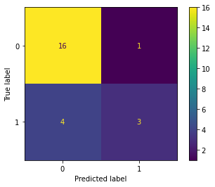
Procedamos a calcular la matriz de confusión.
Por definición, la matriz de confusión \(C\) es tal que \(C_{i, j}\) es igual al número de observaciones conocidas en el grupo \(i\) y predecidas en el grupo \(j\).
from sklearn.metrics import confusion_matrix

cm = confusion_matrix(y, y_pred, labels=[0, 1])
print(cm)
[[16  1]
 [ 4  3]]
pd.DataFrame(cm, index=[0, 1], columns=[0, 1])
| 0 | 1 | |
|---|---|---|
| 0 | 16 | 1 |
| 1 | 4 | 3 |
from sklearn.metrics import plot_confusion_matrix  # New in scikit-learn 0.22

plot_confusion_matrix(Logit, X, y);
Otro ejemplo: Iris Dataset
from sklearn import datasets

iris = datasets.load_iris()
# print(iris.DESCR)
iris_df = (
    pd.DataFrame(iris.data, columns=iris.feature_names)
    .assign(
        target=iris.target,
        target_names=lambda x: x.target.map(dict(zip(range(3), iris.target_names)))
    )
)

iris_df.head()
| sepal length (cm) | sepal width (cm) | petal length (cm) | petal width (cm) | target | target_names | |
|---|---|---|---|---|---|---|
| 0 | 5.1 | 3.5 | 1.4 | 0.2 | 0 | setosa |
| 1 | 4.9 | 3.0 | 1.4 | 0.2 | 0 | setosa |
| 2 | 4.7 | 3.2 | 1.3 | 0.2 | 0 | setosa |
| 3 | 4.6 | 3.1 | 1.5 | 0.2 | 0 | setosa |
| 4 | 5.0 | 3.6 | 1.4 | 0.2 | 0 | setosa |
from sklearn.model_selection import train_test_split
X = iris.data[:,  :2] # we only take the first two features.
y = iris.target

# split dataset
X_train, X_test, y_train, y_test = train_test_split(X, y, test_size=0.2, random_state = 42)

# model
iris_lclf = LogisticRegression()
iris_lclf.fit(X_train, y_train)
LogisticRegression()
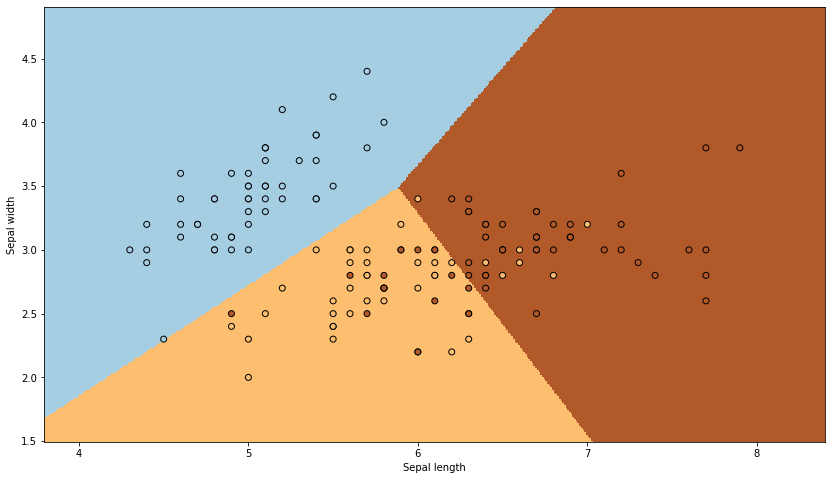
## Inspirado en https://scikit-learn.org/stable/auto_examples/linear_model/plot_iris_logistic.html#sphx-glr-auto-examples-linear-model-plot-iris-logistic-py

plt.figure(figsize=(14, 8))

x_min, x_max = X[:, 0].min() - .5, X[:, 0].max() + .5
y_min, y_max = X[:, 1].min() - .5, X[:, 1].max() + .5

h = .01  # step size in the mesh
xx, yy = np.meshgrid(
    np.arange(x_min, x_max, h),
    np.arange(y_min, y_max, h)
)
Z = iris_lclf.predict(np.c_[xx.ravel(), yy.ravel()])

# Put the result into a color plot
Z = Z.reshape(xx.shape)
plt.pcolormesh(xx, yy, Z, cmap=plt.cm.Paired, shading="auto")

# Plot also the real points
plt.scatter(X[:, 0], X[:, 1], c=y, edgecolors='k', cmap=plt.cm.Paired)
plt.xlabel('Sepal length')
plt.ylabel('Sepal width')
plt.show()
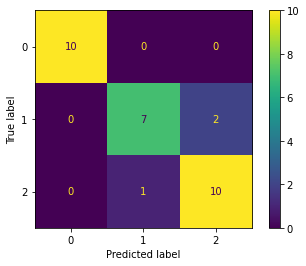
Por otro lado, la predicción debe hacerse con el set de test
y_pred = iris_lclf.predict(X_test)
plot_confusion_matrix(iris_lclf, X_test, y_test);
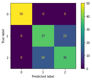
plot_confusion_matrix(iris_lclf, X_train, y_train);
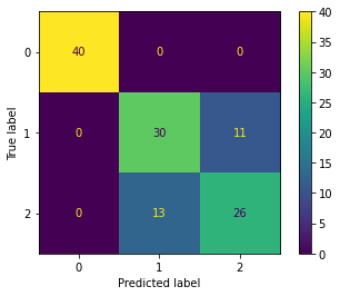
plot_confusion_matrix(iris_lclf, X, y);