Statistical Thinking Foundations#
#these two lines will not change throughout the year
import pandas as pd
import matplotlib.pyplot as plt
url = "https://raw.githubusercontent.com/aoguedao/neural-computing-book/main/data/Diamond%20Prices%202022.csv"
diamonds_df=pd.read_csv(url)
#prints the first 5 rows of the dataframe
print(diamonds_df.head())
#prints the number of columns, attribute headers, data types, and the number of cells in each column (non-null values)
print(diamonds_df.info())
#prints the measures of central tendency for each numerical attribute
print(diamonds_df.describe())
#removes the rows that contain NULL values
diamonds_df = diamonds_df.dropna()
   index  carat      cut color clarity  depth  table  price     x     y     z
0     66   0.28    Ideal     G    VVS2   61.4   56.0    553  4.19  4.22  2.58
1    127   0.91  Premium     H     SI1   61.4   56.0   2763  6.09  5.97  3.70
2    136   0.63  Premium     E    VVS1   60.9   60.0   2765  5.52  5.55  3.37
3    267   0.70  Premium     F     VS1   62.1   60.0   2792  5.71  5.65  3.53
4    324   1.04  Premium     G      I1   62.2   58.0   2801  6.46  6.41  4.00
<class 'pandas.core.frame.DataFrame'>
RangeIndex: 1000 entries, 0 to 999
Data columns (total 11 columns):
 #   Column   Non-Null Count  Dtype
---  ------   --------------  -----
 0   index    1000 non-null   int64
 1   carat    1000 non-null   float64
 2   cut      1000 non-null   object
 3   color    1000 non-null   object
 4   clarity  1000 non-null   object
 5   depth    1000 non-null   float64
 6   table    1000 non-null   float64
 7   price    1000 non-null   int64
 8   x        1000 non-null   float64
 9   y        1000 non-null   float64
 10  z        1000 non-null   float64
dtypes: float64(6), int64(2), object(3)
memory usage: 86.1+ KB
None
              index        carat       depth      table         price  \
count   1000.000000  1000.000000  1000.00000  1000.0000   1000.000000
mean   27027.194000     0.796700    61.75900    57.2640   3958.510000
std    15476.676775     0.476646     1.59089     2.1373   4056.572693
min       66.000000     0.200000    43.00000    50.0000    361.000000
25%    13241.500000     0.400000    61.10000    56.0000    966.000000
50%    27102.000000     0.700000    61.80000    57.0000   2279.500000
75%    40807.750000     1.030000    62.50000    59.0000   5202.750000
max    53916.000000     3.010000    68.60000    67.0000  18768.000000

                 x            y            z
count  1000.000000  1000.000000  1000.000000
mean      5.725390     5.728820     3.540080
std       1.121673     1.114177     0.696209
min       3.730000     3.680000     2.310000
25%       4.740000     4.750000     2.930000
50%       5.670000     5.680000     3.520000
75%       6.510000     6.502500     4.020000
max       9.360000     9.310000     6.160000
#pulls off the price column of the data frame
all_prices = diamonds_df['price']
#print(all_prices)
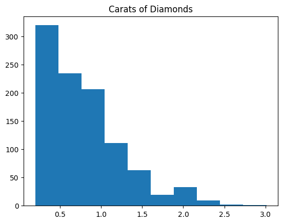
all_carats = diamonds_df['carat']
plt.hist(all_carats)
plt.title('Carats of Diamonds');
plt.show()
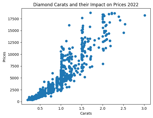
#scatter plot
plt.scatter(all_carats, all_prices)
plt.title("Diamond Carats and their Impact on Prices 2022")
plt.xlabel('Carats')
plt.ylabel('Prices')
plt.show()
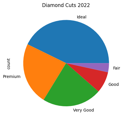
#pie chart
all_cuts = diamonds_df['cut']

all_cuts.value_counts().plot(kind = 'pie')
plt.title("Diamond Cuts 2022")
plt.show()
#storing only the fair cut diamonds
fair = diamonds_df[diamonds_df['cut'] == 'Fair']
#storing only the good cut diamonds
good = diamonds_df[diamonds_df['cut'] == "Good"]
#storing only the ideal cut diamonds
ideal = diamonds_df[diamonds_df['cut'] == 'Ideal']
#storing only the premium cut diamonds
premium = diamonds_df[diamonds_df['cut']== 'Premium']
#storing only the very good cut diamonds
verygood = diamonds_df[diamonds_df['cut'] == 'Very Good']
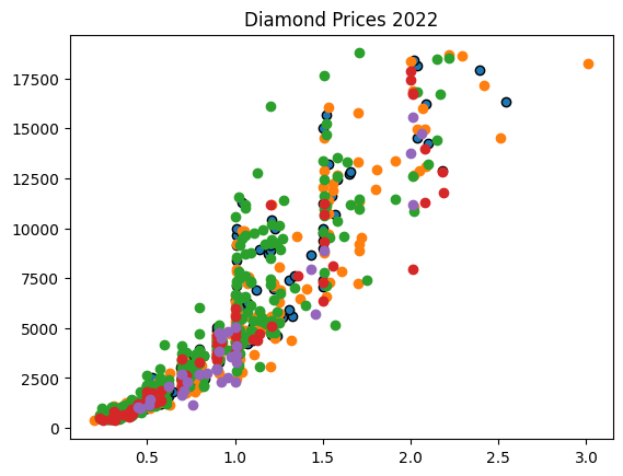
#plotting the multi-variables on a scatter plot
plt.scatter(verygood['carat'], verygood['price'], edgecolor = "black")
plt.scatter(premium['carat'], premium['price'])
plt.scatter(ideal['carat'], ideal['price'])
plt.scatter(good['carat'], good['price'])
plt.scatter(fair['carat'], fair['price'])
plt.title('Diamond Prices 2022')
plt.show()