
Machine Learning - Introduction#
Machine learning is a type of artificial intelligence that teaches machines to identify patterns, make predictions or classify without being explicitly programmed. Instead of telling a computer exactly what to do, you provide it with lots of examples and let it figure out how to solve a problem on its own.
Examples#
Diseases Progression

Image Classification
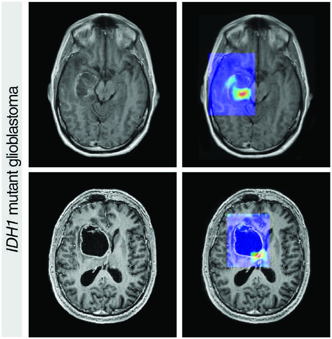
Source: CA Cancer J Clin March/April 2019. doi: 10.3322/caac.21552. CC BY 4.0.
Market Segmentation

Play a videogame

There are three main types of machine learning problems:
Supervised learning: The machine learning algorithm is trained on a labeled dataset, where the input data is paired with the correct output data. The algorithm learns to make predictions by mapping input data to output data.
Unsupervised learning: The machine learning algorithm is trained on an unlabeled dataset, where the input data is not paired with the correct output data. The algorithm learns to identify patterns and relationships in the data on its own.
Reinforcement learning: The machine learning algorithm learns through trial and error by receiving feedback in the form of rewards or penalties. The algorithm learns to make decisions that maximize its reward over time.
Supervised Learning#
Labels can be numeric or categorical, for each case you should use a suitable algorithm.
Regression#
import pandas as pd
from sklearn import datasets

diabetes_data = datasets.load_diabetes(as_frame=True)
print(diabetes_data.DESCR)
.. _diabetes_dataset:

Diabetes dataset
----------------

Ten baseline variables, age, sex, body mass index, average blood
pressure, and six blood serum measurements were obtained for each of n =
442 diabetes patients, as well as the response of interest, a
quantitative measure of disease progression one year after baseline.

**Data Set Characteristics:**

  :Number of Instances: 442

  :Number of Attributes: First 10 columns are numeric predictive values

  :Target: Column 11 is a quantitative measure of disease progression one year after baseline

  :Attribute Information:
      - age     age in years
      - sex
      - bmi     body mass index
      - bp      average blood pressure
      - s1      tc, total serum cholesterol
      - s2      ldl, low-density lipoproteins
      - s3      hdl, high-density lipoproteins
      - s4      tch, total cholesterol / HDL
      - s5      ltg, possibly log of serum triglycerides level
      - s6      glu, blood sugar level

Note: Each of these 10 feature variables have been mean centered and scaled by the standard deviation times the square root of `n_samples` (i.e. the sum of squares of each column totals 1).

Source URL:
https://www4.stat.ncsu.edu/~boos/var.select/diabetes.html

For more information see:
Bradley Efron, Trevor Hastie, Iain Johnstone and Robert Tibshirani (2004) "Least Angle Regression," Annals of Statistics (with discussion), 407-499.
(https://web.stanford.edu/~hastie/Papers/LARS/LeastAngle_2002.pdf)
diabetes_X = diabetes_data.data
diabetes_X
| age | sex | bmi | bp | s1 | s2 | s3 | s4 | s5 | s6 | |
|---|---|---|---|---|---|---|---|---|---|---|
| 0 | 0.038076 | 0.050680 | 0.061696 | 0.021872 | -0.044223 | -0.034821 | -0.043401 | -0.002592 | 0.019907 | -0.017646 |
| 1 | -0.001882 | -0.044642 | -0.051474 | -0.026328 | -0.008449 | -0.019163 | 0.074412 | -0.039493 | -0.068332 | -0.092204 |
| 2 | 0.085299 | 0.050680 | 0.044451 | -0.005670 | -0.045599 | -0.034194 | -0.032356 | -0.002592 | 0.002861 | -0.025930 |
| 3 | -0.089063 | -0.044642 | -0.011595 | -0.036656 | 0.012191 | 0.024991 | -0.036038 | 0.034309 | 0.022688 | -0.009362 |
| 4 | 0.005383 | -0.044642 | -0.036385 | 0.021872 | 0.003935 | 0.015596 | 0.008142 | -0.002592 | -0.031988 | -0.046641 |
| ... | ... | ... | ... | ... | ... | ... | ... | ... | ... | ... |
| 437 | 0.041708 | 0.050680 | 0.019662 | 0.059744 | -0.005697 | -0.002566 | -0.028674 | -0.002592 | 0.031193 | 0.007207 |
| 438 | -0.005515 | 0.050680 | -0.015906 | -0.067642 | 0.049341 | 0.079165 | -0.028674 | 0.034309 | -0.018114 | 0.044485 |
| 439 | 0.041708 | 0.050680 | -0.015906 | 0.017293 | -0.037344 | -0.013840 | -0.024993 | -0.011080 | -0.046883 | 0.015491 |
| 440 | -0.045472 | -0.044642 | 0.039062 | 0.001215 | 0.016318 | 0.015283 | -0.028674 | 0.026560 | 0.044529 | -0.025930 |
| 441 | -0.045472 | -0.044642 | -0.073030 | -0.081413 | 0.083740 | 0.027809 | 0.173816 | -0.039493 | -0.004222 | 0.003064 |
442 rows × 10 columns
diabetes_y = diabetes_data.target
diabetes_y
0      151.0
1       75.0
2      141.0
3      206.0
4      135.0
       ...
437    178.0
438    104.0
439    132.0
440    220.0
441     57.0
Name: target, Length: 442, dtype: float64
from sklearn.linear_model import LinearRegression

model = LinearRegression()
model.fit(diabetes_X, diabetes_y)
print(f"Coefficients:\n {model.coef_.T}\n")
print(f"Score: {model.score(diabetes_X, diabetes_y)}")
Coefficients:
 [ -10.0098663  -239.81564367  519.84592005  324.3846455  -792.17563855
  476.73902101  101.04326794  177.06323767  751.27369956   67.62669218]

Score: 0.5177484222203499
from sklearn.linear_model import Ridge

model = Ridge(alpha=0.1)
model.fit(diabetes_X, diabetes_y)
print(f"Coefficients:\n {model.coef_.T}\n")
print(f"Score: {model.score(diabetes_X, diabetes_y)}")
Coefficients:
 [   1.30870543 -207.19241786  489.69517109  301.76405786  -83.46603399
  -70.8268319  -188.67889782  115.7121356   443.81291747   86.7493154 ]

Score: 0.5125619902742505
from sklearn.linear_model import Lasso

model = Lasso(alpha=0.1)
model.fit(diabetes_X, diabetes_y)
print(f"Coefficients:\n {model.coef_.T}\n")
print(f"Score: {model.score(diabetes_X, diabetes_y)}")
Coefficients:
 [  -0.         -155.3599757   517.18679544  275.07723537  -52.53936509
   -0.         -210.1579914     0.          483.91264753   33.67396468]

Score: 0.5088391185938332
from sklearn.tree import DecisionTreeRegressor

model = DecisionTreeRegressor()
model.fit(diabetes_X, diabetes_y)
# print(f"Coefficients:\n {model.coef_.T}\n")
print(f"Score: {model.score(diabetes_X, diabetes_y)}")
Score: 1.0
Classification#
breast_cancer_data = datasets.load_breast_cancer(as_frame=True)
print(breast_cancer_data.DESCR)
.. _breast_cancer_dataset:

Breast cancer wisconsin (diagnostic) dataset
--------------------------------------------

**Data Set Characteristics:**

    :Number of Instances: 569

    :Number of Attributes: 30 numeric, predictive attributes and the class

    :Attribute Information:
        - radius (mean of distances from center to points on the perimeter)
        - texture (standard deviation of gray-scale values)
        - perimeter
        - area
        - smoothness (local variation in radius lengths)
        - compactness (perimeter^2 / area - 1.0)
        - concavity (severity of concave portions of the contour)
        - concave points (number of concave portions of the contour)
        - symmetry
        - fractal dimension ("coastline approximation" - 1)

        The mean, standard error, and "worst" or largest (mean of the three
        worst/largest values) of these features were computed for each image,
        resulting in 30 features.  For instance, field 0 is Mean Radius, field
        10 is Radius SE, field 20 is Worst Radius.

        - class:
                - WDBC-Malignant
                - WDBC-Benign

    :Summary Statistics:

    ===================================== ====== ======
                                           Min    Max
    ===================================== ====== ======
    radius (mean):                        6.981  28.11
    texture (mean):                       9.71   39.28
    perimeter (mean):                     43.79  188.5
    area (mean):                          143.5  2501.0
    smoothness (mean):                    0.053  0.163
    compactness (mean):                   0.019  0.345
    concavity (mean):                     0.0    0.427
    concave points (mean):                0.0    0.201
    symmetry (mean):                      0.106  0.304
    fractal dimension (mean):             0.05   0.097
    radius (standard error):              0.112  2.873
    texture (standard error):             0.36   4.885
    perimeter (standard error):           0.757  21.98
    area (standard error):                6.802  542.2
    smoothness (standard error):          0.002  0.031
    compactness (standard error):         0.002  0.135
    concavity (standard error):           0.0    0.396
    concave points (standard error):      0.0    0.053
    symmetry (standard error):            0.008  0.079
    fractal dimension (standard error):   0.001  0.03
    radius (worst):                       7.93   36.04
    texture (worst):                      12.02  49.54
    perimeter (worst):                    50.41  251.2
    area (worst):                         185.2  4254.0
    smoothness (worst):                   0.071  0.223
    compactness (worst):                  0.027  1.058
    concavity (worst):                    0.0    1.252
    concave points (worst):               0.0    0.291
    symmetry (worst):                     0.156  0.664
    fractal dimension (worst):            0.055  0.208
    ===================================== ====== ======

    :Missing Attribute Values: None

    :Class Distribution: 212 - Malignant, 357 - Benign

    :Creator:  Dr. William H. Wolberg, W. Nick Street, Olvi L. Mangasarian

    :Donor: Nick Street

    :Date: November, 1995

This is a copy of UCI ML Breast Cancer Wisconsin (Diagnostic) datasets.
https://goo.gl/U2Uwz2

Features are computed from a digitized image of a fine needle
aspirate (FNA) of a breast mass.  They describe
characteristics of the cell nuclei present in the image.

Separating plane described above was obtained using
Multisurface Method-Tree (MSM-T) [K. P. Bennett, "Decision Tree
Construction Via Linear Programming." Proceedings of the 4th
Midwest Artificial Intelligence and Cognitive Science Society,
pp. 97-101, 1992], a classification method which uses linear
programming to construct a decision tree.  Relevant features
were selected using an exhaustive search in the space of 1-4
features and 1-3 separating planes.

The actual linear program used to obtain the separating plane
in the 3-dimensional space is that described in:
[K. P. Bennett and O. L. Mangasarian: "Robust Linear
Programming Discrimination of Two Linearly Inseparable Sets",
Optimization Methods and Software 1, 1992, 23-34].

This database is also available through the UW CS ftp server:

ftp ftp.cs.wisc.edu
cd math-prog/cpo-dataset/machine-learn/WDBC/

.. topic:: References

   - W.N. Street, W.H. Wolberg and O.L. Mangasarian. Nuclear feature extraction
     for breast tumor diagnosis. IS&T/SPIE 1993 International Symposium on
     Electronic Imaging: Science and Technology, volume 1905, pages 861-870,
     San Jose, CA, 1993.
   - O.L. Mangasarian, W.N. Street and W.H. Wolberg. Breast cancer diagnosis and
     prognosis via linear programming. Operations Research, 43(4), pages 570-577,
     July-August 1995.
   - W.H. Wolberg, W.N. Street, and O.L. Mangasarian. Machine learning techniques
     to diagnose breast cancer from fine-needle aspirates. Cancer Letters 77 (1994)
     163-171.
breast_cancer_X = breast_cancer_data.data
breast_cancer_X
| mean radius | mean texture | mean perimeter | mean area | mean smoothness | mean compactness | mean concavity | mean concave points | mean symmetry | mean fractal dimension | ... | worst radius | worst texture | worst perimeter | worst area | worst smoothness | worst compactness | worst concavity | worst concave points | worst symmetry | worst fractal dimension | |
|---|---|---|---|---|---|---|---|---|---|---|---|---|---|---|---|---|---|---|---|---|---|
| 0 | 17.99 | 10.38 | 122.80 | 1001.0 | 0.11840 | 0.27760 | 0.30010 | 0.14710 | 0.2419 | 0.07871 | ... | 25.380 | 17.33 | 184.60 | 2019.0 | 0.16220 | 0.66560 | 0.7119 | 0.2654 | 0.4601 | 0.11890 |
| 1 | 20.57 | 17.77 | 132.90 | 1326.0 | 0.08474 | 0.07864 | 0.08690 | 0.07017 | 0.1812 | 0.05667 | ... | 24.990 | 23.41 | 158.80 | 1956.0 | 0.12380 | 0.18660 | 0.2416 | 0.1860 | 0.2750 | 0.08902 |
| 2 | 19.69 | 21.25 | 130.00 | 1203.0 | 0.10960 | 0.15990 | 0.19740 | 0.12790 | 0.2069 | 0.05999 | ... | 23.570 | 25.53 | 152.50 | 1709.0 | 0.14440 | 0.42450 | 0.4504 | 0.2430 | 0.3613 | 0.08758 |
| 3 | 11.42 | 20.38 | 77.58 | 386.1 | 0.14250 | 0.28390 | 0.24140 | 0.10520 | 0.2597 | 0.09744 | ... | 14.910 | 26.50 | 98.87 | 567.7 | 0.20980 | 0.86630 | 0.6869 | 0.2575 | 0.6638 | 0.17300 |
| 4 | 20.29 | 14.34 | 135.10 | 1297.0 | 0.10030 | 0.13280 | 0.19800 | 0.10430 | 0.1809 | 0.05883 | ... | 22.540 | 16.67 | 152.20 | 1575.0 | 0.13740 | 0.20500 | 0.4000 | 0.1625 | 0.2364 | 0.07678 |
| ... | ... | ... | ... | ... | ... | ... | ... | ... | ... | ... | ... | ... | ... | ... | ... | ... | ... | ... | ... | ... | ... |
| 564 | 21.56 | 22.39 | 142.00 | 1479.0 | 0.11100 | 0.11590 | 0.24390 | 0.13890 | 0.1726 | 0.05623 | ... | 25.450 | 26.40 | 166.10 | 2027.0 | 0.14100 | 0.21130 | 0.4107 | 0.2216 | 0.2060 | 0.07115 |
| 565 | 20.13 | 28.25 | 131.20 | 1261.0 | 0.09780 | 0.10340 | 0.14400 | 0.09791 | 0.1752 | 0.05533 | ... | 23.690 | 38.25 | 155.00 | 1731.0 | 0.11660 | 0.19220 | 0.3215 | 0.1628 | 0.2572 | 0.06637 |
| 566 | 16.60 | 28.08 | 108.30 | 858.1 | 0.08455 | 0.10230 | 0.09251 | 0.05302 | 0.1590 | 0.05648 | ... | 18.980 | 34.12 | 126.70 | 1124.0 | 0.11390 | 0.30940 | 0.3403 | 0.1418 | 0.2218 | 0.07820 |
| 567 | 20.60 | 29.33 | 140.10 | 1265.0 | 0.11780 | 0.27700 | 0.35140 | 0.15200 | 0.2397 | 0.07016 | ... | 25.740 | 39.42 | 184.60 | 1821.0 | 0.16500 | 0.86810 | 0.9387 | 0.2650 | 0.4087 | 0.12400 |
| 568 | 7.76 | 24.54 | 47.92 | 181.0 | 0.05263 | 0.04362 | 0.00000 | 0.00000 | 0.1587 | 0.05884 | ... | 9.456 | 30.37 | 59.16 | 268.6 | 0.08996 | 0.06444 | 0.0000 | 0.0000 | 0.2871 | 0.07039 |
569 rows × 30 columns
breast_cancer_y = breast_cancer_data.target
breast_cancer_y
0      0
1      0
2      0
3      0
4      0
      ..
564    0
565    0
566    0
567    0
568    1
Name: target, Length: 569, dtype: int64
from sklearn.linear_model import LogisticRegression

model = LogisticRegression(max_iter=10000)
model.fit(breast_cancer_X, breast_cancer_y)
print(f"Coefficients:\n {model.coef_}\n")
print(f"Score: {model.score(breast_cancer_X, breast_cancer_y)}")
Coefficients:
 [[ 0.97155351  0.17563154 -0.26255918  0.02235406 -0.17542576 -0.208396
  -0.5178728  -0.29039348 -0.25755614 -0.02809376 -0.06933213  1.24550348
   0.15054852 -0.110651   -0.02503941  0.07211855 -0.02753487 -0.037132
  -0.03238054  0.01476302  0.17889937 -0.43120065 -0.11444469 -0.01354467
  -0.35273091 -0.65900345 -1.38635246 -0.59469895 -0.69872478 -0.08998117]]

Score: 0.9578207381370826
from sklearn.neighbors import KNeighborsClassifier

model = KNeighborsClassifier()
model.fit(breast_cancer_X, breast_cancer_y)
print(f"Score: {model.score(breast_cancer_X, breast_cancer_y)}")
Score: 0.9472759226713533
from sklearn.tree import DecisionTreeClassifier

model = DecisionTreeClassifier()
model.fit(breast_cancer_X, breast_cancer_y)
print(f"Score: {model.score(breast_cancer_X, breast_cancer_y)}")
Score: 1.0
Unsupervised Learning#
Clustering#
filepath = "https://raw.githubusercontent.com/aoguedao/gmu-casbbi-nrt/main/data/gapminder.csv"
data = pd.read_csv(filepath, usecols=[1, 4, 5, 6])
data.head()
| country | continent | life_exp | gdp_cap | |
|---|---|---|---|---|
| 0 | Afghanistan | Asia | 43.828 | 974.580338 |
| 1 | Albania | Europe | 76.423 | 5937.029526 |
| 2 | Algeria | Africa | 72.301 | 6223.367465 |
| 3 | Angola | Africa | 42.731 | 4797.231267 |
| 4 | Argentina | Americas | 75.320 | 12779.379640 |
from sklearn.cluster import KMeans

K = 3
kmeans = KMeans(n_clusters=K)
X = data.drop(columns=["country", "continent"])
kmeans.fit(X)
/home/alonsolml/mambaforge/envs/casbbi-nrt-ds/lib/python3.11/site-packages/sklearn/cluster/_kmeans.py:870: FutureWarning: The default value of `n_init` will change from 10 to 'auto' in 1.4. Set the value of `n_init` explicitly to suppress the warning
  warnings.warn(
KMeans(n_clusters=3)In a Jupyter environment, please rerun this cell to show the HTML representation or trust the notebook.
On GitHub, the HTML representation is unable to render, please try loading this page with nbviewer.org.
KMeans(n_clusters=3)
data["label"] = kmeans.labels_
data.head()
| country | continent | life_exp | gdp_cap | label | |
|---|---|---|---|---|---|
| 0 | Afghanistan | Asia | 43.828 | 974.580338 | 1 |
| 1 | Albania | Europe | 76.423 | 5937.029526 | 1 |
| 2 | Algeria | Africa | 72.301 | 6223.367465 | 1 |
| 3 | Angola | Africa | 42.731 | 4797.231267 | 1 |
| 4 | Argentina | Americas | 75.320 | 12779.379640 | 0 |
data.query("label == 0")
| country | continent | life_exp | gdp_cap | label | |
|---|---|---|---|---|---|
| 4 | Argentina | Americas | 75.320 | 12779.379640 | 0 |
| 13 | Botswana | Africa | 50.728 | 12569.851770 | 0 |
| 14 | Brazil | Americas | 72.390 | 9065.800825 | 0 |
| 15 | Bulgaria | Europe | 73.005 | 10680.792820 | 0 |
| 23 | Chile | Americas | 78.553 | 13171.638850 | 0 |
| 29 | Costa Rica | Americas | 78.782 | 9645.061420 | 0 |
| 31 | Croatia | Europe | 75.748 | 14619.222720 | 0 |
| 32 | Cuba | Americas | 78.273 | 8948.102923 | 0 |
| 33 | Czech Republic | Europe | 76.486 | 22833.308510 | 0 |
| 40 | Equatorial Guinea | Africa | 51.579 | 12154.089750 | 0 |
| 45 | Gabon | Africa | 56.735 | 13206.484520 | 0 |
| 56 | Hungary | Europe | 73.338 | 18008.944440 | 0 |
| 60 | Iran | Asia | 70.964 | 11605.714490 | 0 |
| 70 | Korea, Rep. | Asia | 78.623 | 23348.139730 | 0 |
| 72 | Lebanon | Asia | 71.993 | 10461.058680 | 0 |
| 75 | Libya | Africa | 73.952 | 12057.499280 | 0 |
| 78 | Malaysia | Asia | 74.241 | 12451.655800 | 0 |
| 81 | Mauritius | Africa | 72.801 | 10956.991120 | 0 |
| 82 | Mexico | Americas | 76.195 | 11977.574960 | 0 |
| 84 | Montenegro | Europe | 74.543 | 9253.896111 | 0 |
| 96 | Oman | Asia | 75.640 | 22316.192870 | 0 |
| 98 | Panama | Americas | 75.537 | 9809.185636 | 0 |
| 102 | Poland | Europe | 75.563 | 15389.924680 | 0 |
| 103 | Portugal | Europe | 78.098 | 20509.647770 | 0 |
| 104 | Puerto Rico | Americas | 78.746 | 19328.709010 | 0 |
| 106 | Romania | Europe | 72.476 | 10808.475610 | 0 |
| 109 | Saudi Arabia | Asia | 72.777 | 21654.831940 | 0 |
| 111 | Serbia | Europe | 74.002 | 9786.534714 | 0 |
| 114 | Slovak Republic | Europe | 74.663 | 18678.314350 | 0 |
| 117 | South Africa | Africa | 49.339 | 9269.657808 | 0 |
| 129 | Trinidad and Tobago | Americas | 69.819 | 18008.509240 | 0 |
| 131 | Turkey | Europe | 71.777 | 8458.276384 | 0 |
| 135 | Uruguay | Americas | 76.384 | 10611.462990 | 0 |
| 136 | Venezuela | Americas | 73.747 | 11415.805690 | 0 |
data.query("label == 1")
| country | continent | life_exp | gdp_cap | label | |
|---|---|---|---|---|---|
| 0 | Afghanistan | Asia | 43.828 | 974.580338 | 1 |
| 1 | Albania | Europe | 76.423 | 5937.029526 | 1 |
| 2 | Algeria | Africa | 72.301 | 6223.367465 | 1 |
| 3 | Angola | Africa | 42.731 | 4797.231267 | 1 |
| 8 | Bangladesh | Asia | 64.062 | 1391.253792 | 1 |
| ... | ... | ... | ... | ... | ... |
| 137 | Vietnam | Asia | 74.249 | 2441.576404 | 1 |
| 138 | West Bank and Gaza | Asia | 73.422 | 3025.349798 | 1 |
| 139 | Yemen, Rep. | Asia | 62.698 | 2280.769906 | 1 |
| 140 | Zambia | Africa | 42.384 | 1271.211593 | 1 |
| 141 | Zimbabwe | Africa | 43.487 | 469.709298 | 1 |
80 rows × 5 columns
data.query("label == 2")
| country | continent | life_exp | gdp_cap | label | |
|---|---|---|---|---|---|
| 5 | Australia | Oceania | 81.235 | 34435.36744 | 2 |
| 6 | Austria | Europe | 79.829 | 36126.49270 | 2 |
| 7 | Bahrain | Asia | 75.635 | 29796.04834 | 2 |
| 9 | Belgium | Europe | 79.441 | 33692.60508 | 2 |
| 20 | Canada | Americas | 80.653 | 36319.23501 | 2 |
| 34 | Denmark | Europe | 78.332 | 35278.41874 | 2 |
| 43 | Finland | Europe | 79.313 | 33207.08440 | 2 |
| 44 | France | Europe | 80.657 | 30470.01670 | 2 |
| 47 | Germany | Europe | 79.406 | 32170.37442 | 2 |
| 49 | Greece | Europe | 79.483 | 27538.41188 | 2 |
| 55 | Hong Kong, China | Asia | 82.208 | 39724.97867 | 2 |
| 57 | Iceland | Europe | 81.757 | 36180.78919 | 2 |
| 62 | Ireland | Europe | 78.885 | 40675.99635 | 2 |
| 63 | Israel | Asia | 80.745 | 25523.27710 | 2 |
| 64 | Italy | Europe | 80.546 | 28569.71970 | 2 |
| 66 | Japan | Asia | 82.603 | 31656.06806 | 2 |
| 71 | Kuwait | Asia | 77.588 | 47306.98978 | 2 |
| 90 | Netherlands | Europe | 79.762 | 36797.93332 | 2 |
| 91 | New Zealand | Oceania | 80.204 | 25185.00911 | 2 |
| 95 | Norway | Europe | 80.196 | 49357.19017 | 2 |
| 113 | Singapore | Asia | 79.972 | 47143.17964 | 2 |
| 115 | Slovenia | Europe | 77.926 | 25768.25759 | 2 |
| 118 | Spain | Europe | 80.941 | 28821.06370 | 2 |
| 122 | Sweden | Europe | 80.884 | 33859.74835 | 2 |
| 123 | Switzerland | Europe | 81.701 | 37506.41907 | 2 |
| 125 | Taiwan | Asia | 78.400 | 28718.27684 | 2 |
| 133 | United Kingdom | Europe | 79.425 | 33203.26128 | 2 |
| 134 | United States | Americas | 78.242 | 42951.65309 | 2 |
Machine Learning is not always the solution!#
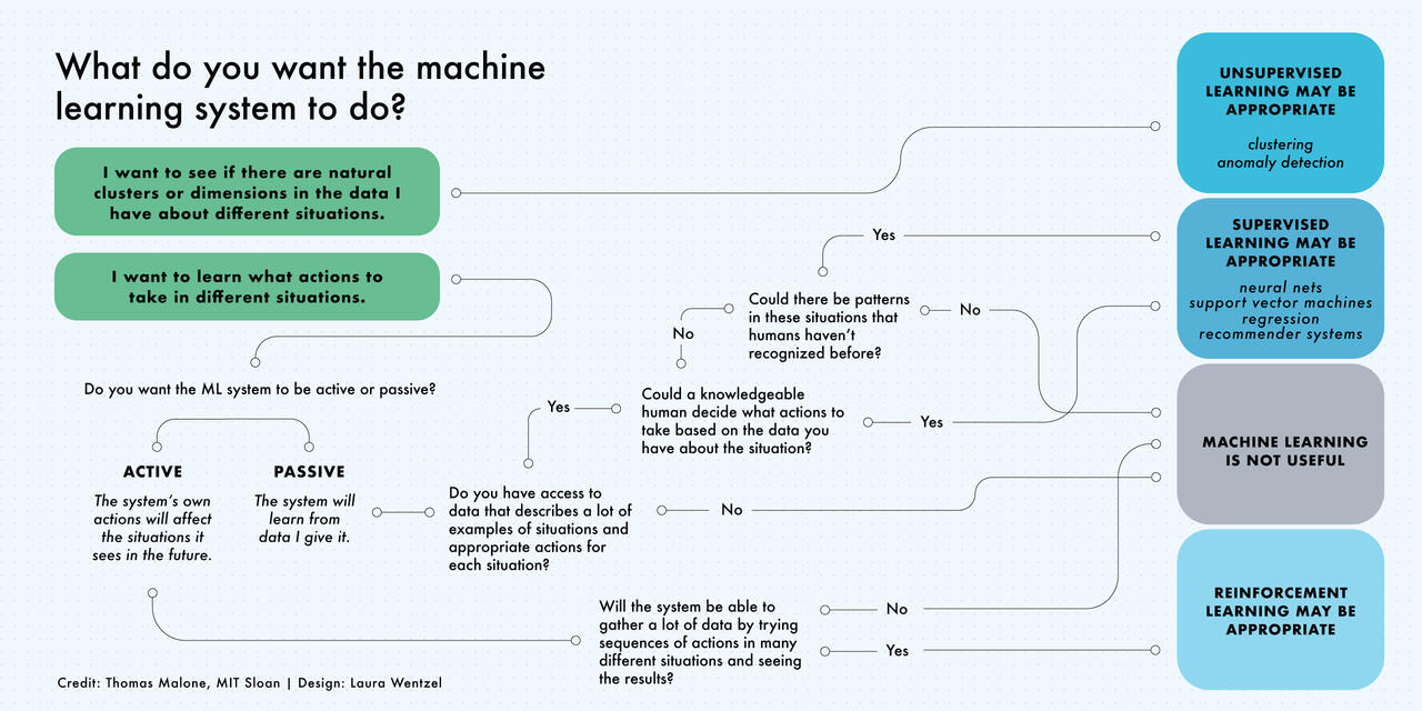
Source: https://mitsloan.mit.edu/ideas-made-to-matter/machine-learning-explained